Learn interpreting audio measurements with Cavern

What is on this page?

Plain and simple: everything you need to know to assemble your very own audio measurement tool, then the exact steps of how to combine these concepts. If you only need the exact operations for drawing a frequency response, skip to the TL;DR chapter.

Fourier transform simplified

We will be working in Fourier space, which means we will use a specific formula to transform the samples of the measurement into complex offsets for each frequency band. The exact math is not important right now, there are industry standard libraries for that like fftw. Cavern has its own heavily optimized FFT (Fast Fourier Transform) implementation for portability. When we Fourier transform a set of samples, the results will be complex numbers in the form of Re(x) + Im(x) * i, where Re(x) is the real part and Im(x) is the imaginary part. Each complex number corresponds to a band. To see which band, just equally divide the bands to the sampling rate. In a very small example, let's say we had 4 samples and the sampling rate is 1000. Then, the bands will be 0 Hz, 250 Hz, 500 Hz, and 750 Hz. There is no 1000 Hz, the sample rate as a band is always missing. In reality, we work with much more bands for good precision. In the example, these bands also correspond to the sine waves that would take 0, 1, 2, and 3 cycles in the sampled timeslot of the audio. The frequencies work out this way too: if we take 4 samples out of a second of content at 1000 Hz, which is 1000 samples, that accounts for 4/1000th or 1/250th of a second, so a single wavelength fitting there would be 250 Hz, exactly what we've seen.

So we have a complex number for each frequency band, what do they mean? We've split the audio we're working with into its components, each of which is some kind of sine wave. The complex numbers describe their properties, just not with their raw components. The first property we need is the amplitude (also called the absolute value): sqrt(Re(x)² + Im(x)²). It describes how much of a given band there is in the signal. 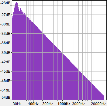If we graph it, we get how loud the signal is at each frequency, which is exactly how we previously defined the frequency response. So, the frequency response for a signal in short is abs(fft(signal)). Another thing is the phase, how much offset there is compared to a single cycle in radians, basically how much we pushed the signal out to the right, which appeared again from the left. Yeah, Fourier transforms are circular, keep this in mind when designing something like subsample precision delays. Phase is calculated by atan2(Im(x), Re(x)). One important thing to note is phase correction is not as simple as rotating these complex numbers, this can completely break the signal by distorting the complex waveforms these bands are the components of, inducing hums. Even amplitude modification is not as easy as just multiplying the complex numbers and doing an inverse Fourier transform to get the modified signal back. The only case where that works is if we EQ a Dirac-delta.

Swept sine signals

We noted that we need to spread the frequencies in time to achieve a signal to noise ratio that is usable for measurements. One already existing concept is the swept sine wave (or sweep for short), which modifies a sine wave to increase in frequency between a start and end frequency, increasing with a constant octave range, so logarithmically. Linear sweeps also work, but we will draw logarithmic graphs, this is how we get optimal performance for it. Cavern generates sweeps the following way:

Calculate the chirpyness, or how fast the frequency change increases: (end frequency - start frequency) ^ (sample rate / signal length in samples).
For each sample, set its value to sin[2 * pi * start frequency * (chirpyness ^ (sample index / sample rate) - 1) / ln(chirpyness)].

If we Fourier transform this signal, we can see that its spectrum is not linear, not even resembling the 3 dB/octave decrease of pink noise as the logarithmic power distribution would suggest:

This is not a perfect line, but a bit wobbly, so we have to account for that with the deconvolution, but first, we need to learn what normal convolution is.

This is only an advertisement and keeps Cavern free.

Convolution

We talked about FIR filters being practically an impulse response, more specifically the result of what would happen with a Dirac-delta if the changes the filter describes were to be performed on it. The Dirac-delta is the identity operator in Fourier-space, everything multiplied by the Dirac-delta's FFT stays what it was, so the Dirac-delta is the perfect impulse response. It's a constant 1 + 0 * i for each band. Thus, comes the idea, if we multiply any signal in Fourier-space with an impulse response, we could apply the changes of the filter to that signal. This is not the definition of convolution, but the computationally optimized version of it. To apply a filter's impulse response on a signal, or to convolve the signal with the filter, first, perform a Fourier transform on both, then multiply them together band by band, then invert the Fourier transform on the result to get the modified signal back. Essentially this is how convolution filters are applied.

Because convolution results by definition are twice as long as the inputs, keep in mind to pad them with silence. This only applies to convolution, not to deconvolution. When performing convolutions in real time, the latency should be low, so the signal has to be convolved at very few sample intervals, let's say at every 256 samples. In this case, it needs a lot of padding to be convolved with a regular sized convolution filter of 65536 samples, and will have a lot of increased length. This is not a problem, just keep the remaining samples, and add the next 256 samples of the result to the next frame of 256 samples of input data and so on.

Deconvolution

We've seen that the excitement signal convolved with an impulse response of a filter or a system is the excitement response. This works backwards too, and the two sides of the multiplication are interchangeable: if we know at least one of them and the response, we can get the other by division. For a measurement, we know the excitement signal and the excitement response, we just need the impulse response. We have everything, work backwards from what we know about convolution, in small steps. First, we work in Fourier-space, so Fourier transform both of our inputs. Because convolution was a multiplication, let's divide them in this case: FFT(excitement response) / FFT(excitement signal). This operation is still in Fourier-space, so we need an inverse Fourier transform to get the impulse response. There are more information in the division, however. Practically, we are done with the evaluation, because this is what we call a transfer function, which means this describes the changes to each frequency band for our input signals. This includes the changes in amplitude, so if we just plot the amplitude of each band in the transfer function, we get the frequency response. Additionally, if we plot the phase of each band, we get the phase response.

Another very good use for the deconvolution is that you can remove the effect of components one by one from the result. Imagine your audio system: your amplifier's distortions (its impulse response) get technically convolved with the speakers' distortion, and then with the room's distortions. If you can measure one individually, you can get the others back. So if you measure your amplifiers individually and the speakers with a calibrated amplification chain in open air, you can technically deconvolve the amplifier and speaker response from the result to get back the impulse response of your room. That would contain the "EQ" of your room too, which is called a room curve.

TL;DR

With all of our tools combined, we can use them to create an excitement signal, and process the recorded excitement response to display either the impulse response or the frequency response:

Create the excitement signal as a swept sine.
Play the excitement signal on the system, and record the excitement response.
Calculate the transfer function: FFT(excitement response) / FFT(excitement signal).

From here, you have many options:

Calculate the frequency response with abs(transfer function).
Calculate the phase response with atan2(transfer function).
Calculate the impulse response with Re(IFFT(transfer function)).

Congratulations, now you have your very own acoustic measurement software!